🤖 Ask PyProf.

🗑 −

▶ שלח

⏳ ממתין...

שימוש ב־Pandas יחד עם Matplotlib ו־NumPy

Pandas נוחה מאוד לארגון ולבחירה של נתונים, אבל לעיתים נרצה להשתמש בספריות אחרות על אותם נתונים. בדוגמה זו נראה שני חיבורים חשובים:

• שימוש ב־Matplotlib כדי להציג שאלה כימית בצורה גרפית.

• המרה של עמודות Pandas למערכי NumPy בעזרת .to_numpy().

Note

אפשר להוריד את קובץ הנתונים לעבודה עצמאית: compound_phase_points.csv.

import pandas as pd
import numpy as np
import matplotlib.pyplot as plt

pd.options.display.max_rows = 20

df = pd.read_csv("files/compound_phase_points.csv")
display(df)

	compound	formula	family	molar_mass_g_mol	melting_point_C	boiling_point_C	polarity
0	water	H2O	inorganic	18.02	0.0	100.0	polar
1	methanol	CH4O	alcohol	32.04	-97.6	64.7	polar
2	ethanol	C2H6O	alcohol	46.07	-114.1	78.4	polar
3	1-propanol	C3H8O	alcohol	60.10	-126.0	97.2	polar
4	acetone	C3H6O	ketone	58.08	-94.7	56.1	polar
5	diethyl ether	C4H10O	ether	74.12	-116.3	34.6	weakly polar
6	hexane	C6H14	alkane	86.18	-95.0	68.7	nonpolar
7	heptane	C7H16	alkane	100.20	-90.6	98.4	nonpolar
8	benzene	C6H6	aromatic	78.11	5.5	80.1	nonpolar
9	toluene	C7H8	aromatic	92.14	-95.0	110.6	nonpolar
10	acetic acid	C2H4O2	carboxylic acid	60.05	16.6	118.1	polar
11	chloroform	CHCl3	halogenated	119.38	-63.5	61.2	weakly polar
12	ethane	C2H6	alkane	30.07	-182.8	-88.6	nonpolar
13	butane	C4H10	alkane	58.12	-138.3	-0.5	nonpolar
14	naphthalene	C10H8	aromatic	128.17	80.2	218.0	nonpolar
15	benzoic acid	C7H6O2	carboxylic acid	122.12	122.4	249.2	polar

גרף עמודות: אילו חומרים רותחים גבוה יותר?

כאשר רוצים להשוות ערך מספרי בין קטגוריות, גרף עמודות הוא בחירה טבעית. כאן כל קטגוריה היא תרכובת, והערך הוא נקודת הרתיחה שלה.

שימו לב שהשורה sort_values בהמשך לא מסננת חומרים מהטבלה. היא רק משנה את סדר השורות, כך שהתרכובות יוצגו מהרתיחה הנמוכה ביותר לגבוהה ביותר. כל התרכובות שנמצאות ב־df מופיעות בגרף.

boiling_sorted = df.sort_values("boiling_point_C")
bar_colors = np.where(boiling_sorted["boiling_point_C"] < 25, "tab:orange", "tab:blue")

fig, ax = plt.subplots(figsize=(9, 7.5))
ax.barh(boiling_sorted["compound"], boiling_sorted["boiling_point_C"], color=bar_colors)
ax.axvline(25, color="0.4", linestyle="--", linewidth=1, label="25°C")

for compound, boiling in zip(boiling_sorted["compound"], boiling_sorted["boiling_point_C"]):
    if boiling >= 0:
        x_text = boiling + 4
        ha = "left"
    else:
        x_text = boiling - 5
        ha = "right"
    ax.text(x_text, compound, f"{boiling:g}", va="center", ha=ha, fontsize=8)

ax.set_xlim(-130, 280)
ax.set_xlabel("Boiling point (°C)")
ax.set_ylabel("Compound")
ax.set_title("Boiling points of selected compounds")
ax.legend()
ax.grid(axis="x", alpha=0.3)
plt.show()

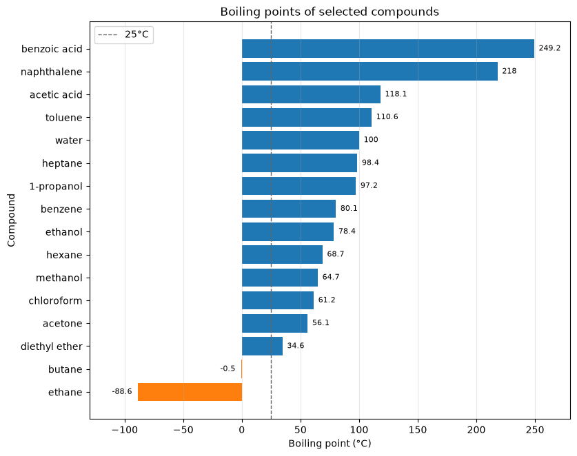
הסידור לפי נקודת הרתיחה מקל על הקריאה: אפשר לראות מיד ש־diethyl ether רותח בטמפרטורה נמוכה יחסית, וש־acetic acid נמצאת בקצה הגבוה של הטבלה. זהו שימוש טוב בגרף: הוא עונה על שאלה אחת ברורה.

המרה למערכי NumPy

פונקציות רבות במדע חישובי מקבלות מערכי NumPy. עמודת Pandas היא Series, ואפשר להמיר אותה למערך בעזרת .to_numpy(). כאן נשתמש בשתי עמודות מספריות שיש להן משמעות כימית ברורה: נקודת ההתכה ונקודת הרתיחה.

melting_point = df["melting_point_C"].to_numpy()
boiling_point = df["boiling_point_C"].to_numpy()
compound_names = df["compound"].to_numpy()

print(type(melting_point))
print(compound_names)
print(melting_point)
print(boiling_point)

<class 'numpy.ndarray'>
['water' 'methanol' 'ethanol' '1-propanol' 'acetone' 'diethyl ether'
 'hexane' 'heptane' 'benzene' 'toluene' 'acetic acid' 'chloroform'
 'ethane' 'butane' 'naphthalene' 'benzoic acid']
[   0.   -97.6 -114.1 -126.   -94.7 -116.3  -95.   -90.6    5.5  -95.
   16.6  -63.5 -182.8 -138.3   80.2  122.4]
[100.   64.7  78.4  97.2  56.1  34.6  68.7  98.4  80.1 110.6 118.1  61.2
 -88.6  -0.5 218.  249.2]

כעת melting_point ו־boiling_point הם מערכי NumPy רגילים. אפשר לבצע עליהם חישובים לוגיים בדיוק כמו שלמדנו ב־NumPy.

room_temperature_C = 25

is_liquid = (
    (melting_point < room_temperature_C)
    & (boiling_point > room_temperature_C)
)

print(is_liquid)

[ True  True  True  True  True  True  True  True  True  True  True  True
 False False False False]

המערך is_liquid מכיל ערכי אמת/שקר. כל ערך עונה על אותה שאלה עבור תרכובת אחת: האם 25°C נמצאת בין נקודת ההתכה לבין נקודת הרתיחה?

גרף פאזה פשוט

נשתמש במערכי NumPy שיצרנו כדי לצייר גרף של נקודת רתיחה מול נקודת התכה. הקווים האפורים מסמנים את 25°C. תרכובות שנמצאות משמאל לקו האנכי ומעל הקו האופקי צפויות להיות נוזליות בטמפרטורת החדר.

fig, ax = plt.subplots(figsize=(6, 5))

ax.scatter(
    melting_point[is_liquid],
    boiling_point[is_liquid],
    label="Liquid at 25°C",
)
ax.scatter(
    melting_point[~is_liquid],
    boiling_point[~is_liquid],
    label="Not liquid at 25°C",
)

for name, melting, boiling in zip(compound_names, melting_point, boiling_point):
    ax.annotate(name, (melting, boiling), xytext=(4, 3), textcoords="offset points", fontsize=8)

ax.axvline(room_temperature_C, color="0.5", linestyle="--", linewidth=1)
ax.axhline(room_temperature_C, color="0.5", linestyle="--", linewidth=1)
ax.set_xlabel("Melting point (°C)")
ax.set_ylabel("Boiling point (°C)")
ax.set_title("Phase at room temperature")
ax.legend()
ax.grid(alpha=0.3)
plt.show()

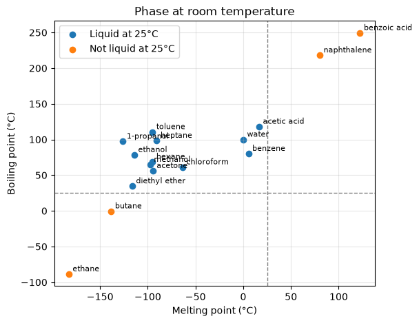
הגרף הזה פחות מנסה למצוא “חוק” כללי, ויותר עוזר לקרוא את הטבלה. הוא מראה את אותו תנאי שכתבנו בקוד: חומר נוזלי בטמפרטורת החדר אם נקודת ההתכה שלו נמוכה מ־25°C ונקודת הרתיחה שלו גבוהה מ־25°C.

כרגע התוצאה נמצאת רק במערך NumPy בשם is_liquid. אם נרצה להמשיך לעבוד עם התוצאה כחלק מהטבלה, למשל למיין, לסנן, להציג או לשמור אותה, כדאי להחזיר אותה ל־DataFrame כעמודה חדשה. כך כל תרכובת מקבלת גם את הסיווג שחישבנו עבורה.

df["liquid_at_25_C"] = is_liquid

display(df[["compound", "melting_point_C", "boiling_point_C", "liquid_at_25_C"]])

	compound	melting_point_C	boiling_point_C	liquid_at_25_C
0	water	0.0	100.0	True
1	methanol	-97.6	64.7	True
2	ethanol	-114.1	78.4	True
3	1-propanol	-126.0	97.2	True
4	acetone	-94.7	56.1	True
5	diethyl ether	-116.3	34.6	True
6	hexane	-95.0	68.7	True
7	heptane	-90.6	98.4	True
8	benzene	5.5	80.1	True
9	toluene	-95.0	110.6	True
10	acetic acid	16.6	118.1	True
11	chloroform	-63.5	61.2	True
12	ethane	-182.8	-88.6	False
13	butane	-138.3	-0.5	False
14	naphthalene	80.2	218.0	False
15	benzoic acid	122.4	249.2	False

כך מתקבל רצף עבודה נפוץ: Pandas לארגון הנתונים, NumPy לחישוב מספרי או לוגי, ו־Matplotlib להצגה גרפית של השאלה המדעית.