Libraries: Pandas (1.5 weeks)

Libraries: Pandas (1.5 weeks)#

Python Programming for Engineers#

Tel-Aviv University / 0509-1820 / Fall 2025-2026#

Agenda: Pandas#

Introduction
Counteries datasets
- Data fetching
- Data cleaning
- Data analysis

Introduction to Pandas#

import pandas as pd
import numpy as np # This is not mandatory for using Pandas
import utils.load_auxilary_files # This will load the files used for this notebook

['orders_4_2024.csv', 'witcher_2.csv', 'evil_morty_change_noised.png', 'StudentsGrades.csv', 'dog.png', 'notebook_resources.zip', 'erosion_2.png', 'dialation_2.png', 'ship.png', 'ex1.csv', 'ex2.csv', 'countries-of-the-world.csv', 'koala.png', 'orders_2_2024.csv', 'hello', 'dialation.png', '__MACOSX', 'baby.png', 'evil_morty_change_3.png', 'evil_morty_segmentation.png', 'woman_noised.png', 'orders_3_2024.csv', 'evil_morty_change.png', 'erosion.png', 'evil_morty_1.png', 'dog_noised.png', 'witcher_1.csv', 'products2.csv']

Basic operations (1)#

Read a dataframe#

df = pd.read_csv("files/countries-of-the-world.csv")

print('"Raw" display. This is how dataframes usually displayed on console')
print(df)

"Raw" display. This is how dataframes usually displayed on console
          Country              Region   Population     Area  Pop. Density  \
        Angola  SUB-SAHARAN AFRICA   12127071.0  1246700           9.7   
   Afghanistan                ASIA          NaN   647500          15.3   
  Sierra Leone  SUB-SAHARAN AFRICA    6005250.0    71740          83.7   
    Mozambique  SUB-SAHARAN AFRICA   19686505.0   801590          24.6   
       Liberia  SUB-SAHARAN AFRICA    3042004.0   111370          27.3   
..            ...                 ...          ...      ...           ...   
     Iceland      WESTERN EUROPE     299388.0   103000           2.9   
       Japan                ASIA  127463611.0   377835         337.4   
   Hong Kong                ASIA    6940432.0     1092        6355.7   
      Sweden      WESTERN EUROPE    9016596.0   449964          20.0   
   Singapore                ASIA    4492150.0      693        6482.2   

     Infant mortality (per 1000 births)  GDP ($ per capita)  Birthrate  \
                              191.19              1900.0      45.11   
                              163.07               700.0      46.60   
                              143.64               500.0      45.76   
                              130.79              1200.0      35.18   
                              128.87              1000.0      44.77   
..                                  ...                 ...        ...   
                              3.31             30900.0      13.64   
                              3.26             28200.0       9.37   
                              2.97             28800.0       7.29   
                              2.77             26800.0      10.27   
                              2.29             23700.0       9.34   

     Deathrate  
      24.20  
      20.34  
      23.03  
      21.35  
      23.10  
..         ...  
     6.72  
     9.16  
     6.29  
    10.31  
     4.28  

[224 rows x 9 columns]

print('formatted display (only in Jupyter Notebooks)')
display(df)

formatted display (only in Jupyter Notebooks)

	Country	Region	Population	Area	Pop. Density	Infant mortality (per 1000 births)	GDP ($ per capita)	Birthrate	Deathrate
0	Angola	SUB-SAHARAN AFRICA	12127071.0	1246700	9.7	191.19	1900.0	45.11	24.20
1	Afghanistan	ASIA	NaN	647500	15.3	163.07	700.0	46.60	20.34
2	Sierra Leone	SUB-SAHARAN AFRICA	6005250.0	71740	83.7	143.64	500.0	45.76	23.03
3	Mozambique	SUB-SAHARAN AFRICA	19686505.0	801590	24.6	130.79	1200.0	35.18	21.35
4	Liberia	SUB-SAHARAN AFRICA	3042004.0	111370	27.3	128.87	1000.0	44.77	23.10
...	...	...	...	...	...	...	...	...	...
219	Iceland	WESTERN EUROPE	299388.0	103000	2.9	3.31	30900.0	13.64	6.72
220	Japan	ASIA	127463611.0	377835	337.4	3.26	28200.0	9.37	9.16
221	Hong Kong	ASIA	6940432.0	1092	6355.7	2.97	28800.0	7.29	6.29
222	Sweden	WESTERN EUROPE	9016596.0	449964	20.0	2.77	26800.0	10.27	10.31
223	Singapore	ASIA	4492150.0	693	6482.2	2.29	23700.0	9.34	4.28

224 rows × 9 columns

print(df.columns)

Index(['Country', 'Region', 'Population', 'Area', 'Pop. Density',
       'Infant mortality (per 1000 births)', 'GDP ($ per capita)', 'Birthrate',
       'Deathrate'],
      dtype='str')

`[]`, `loc[]` and `iloc[]`#

print(df["Country"])

          Angola
     Afghanistan
    Sierra Leone
      Mozambique
         Liberia
           ...     
       Iceland
         Japan
     Hong Kong
        Sweden
     Singapore
Name: Country, Length: 224, dtype: str

print(df["Population"].dtype)

float64

print(df["Population"] / df["Area"])

       9.727337
            NaN
      83.708531
      24.559320
      27.314393
          ...     
     2.906680
   337.352577
  6355.706960
    20.038483
  6482.178932
Length: 224, dtype: float64

df = pd.DataFrame(np.array([[1, 2, 3], [4, 5, 6], [7, 8, 9]]),
                  columns=['a', 'b', 'c'],index=[3, 4, 5])
display(df)

	a	b	c
3	1	2	3
4	4	5	6
5	7	8	9

display(df.iloc[:,:2]) 

	a	b
3	1	2
4	4	5
5	7	8

display(df.loc[:,:'b']) 

	a	b
3	1	2
4	4	5
5	7	8

Do not get confused between `df[]`, `df.loc[]` and `df.iloc[]`!#

(3): What will be printed? #

df = pd.DataFrame(np.array([[1, 2, 3], [4, 5, 6], [7, 8, 9]]),
                  columns=['a', 'b', 'c'],index=[3, 4, 5])
display(df)

	a	b	c
3	1	2	3
4	4	5	6
5	7	8	9

print(type(df))
print(type(df.iloc[0]))
print(type(df.iloc[:,0]))

<class 'pandas.DataFrame'>
<class 'pandas.Series'>
<class 'pandas.Series'>

Example: Countries dataset#

Analysis steps#

Install pandas with anaconda as described here (via Pycharm) or here (on windows)
Get basic information
Data cleaning – fill missing data
Basic data analysis
Data Visualization - Self learning

1. Get basic information (and some more basic operations)#

Read a csv#

df = pd.read_csv("files/countries-of-the-world.csv")

Write dataframe to csv#

df.to_csv("files/countries-of-the-world_out.csv")

Print the top 3 rows using the `head` function#

display(df.head(3))

	Country	Region	Population	Area	Pop. Density	Infant mortality (per 1000 births)	GDP ($ per capita)	Birthrate	Deathrate
0	Angola	SUB-SAHARAN AFRICA	12127071.0	1246700	9.7	191.19	1900.0	45.11	24.20
1	Afghanistan	ASIA	NaN	647500	15.3	163.07	700.0	46.60	20.34
2	Sierra Leone	SUB-SAHARAN AFRICA	6005250.0	71740	83.7	143.64	500.0	45.76	23.03

Note that NaN on the second row!#

df.info()

<class 'pandas.DataFrame'>
RangeIndex: 224 entries, 0 to 223
Data columns (total 9 columns):
 #   Column                              Non-Null Count  Dtype  
---  ------                              --------------  -----  
 0   Country                             224 non-null    str    
 1   Region                              224 non-null    str    
 2   Population                          220 non-null    float64
 3   Area                                224 non-null    int64  
 4   Pop. Density                        223 non-null    float64
 5   Infant mortality (per 1000 births)  224 non-null    float64
 6   GDP ($ per capita)                  223 non-null    float64
 7   Birthrate                           223 non-null    float64
 8   Deathrate                           222 non-null    float64
dtypes: float64(6), int64(1), str(2)
memory usage: 15.9 KB

2. Data cleaning#

fill missing values#

Option 1: replace nan values with 0 (or any other constant value)#

df=pd.read_csv("files/countries-of-the-world.csv").loc[[0,1,2,3],["Country","Region","Population","Area"]]
display(df)
df = df.fillna(0)
display(df)

	Country	Region	Population	Area
0	Angola	SUB-SAHARAN AFRICA	12127071.0	1246700
1	Afghanistan	ASIA	NaN	647500
2	Sierra Leone	SUB-SAHARAN AFRICA	6005250.0	71740
3	Mozambique	SUB-SAHARAN AFRICA	19686505.0	801590

	Country	Region	Population	Area
0	Angola	SUB-SAHARAN AFRICA	12127071.0	1246700
1	Afghanistan	ASIA	0.0	647500
2	Sierra Leone	SUB-SAHARAN AFRICA	6005250.0	71740
3	Mozambique	SUB-SAHARAN AFRICA	19686505.0	801590

Option 2: replace nan values with the average of the column#

df=pd.read_csv("files/countries-of-the-world.csv").loc[[0,1,2,3],["Country","Region","Population","Area"]]
display(df)
df['Population']=df['Population'].fillna(df.loc[:,'Population'].mean())
print(df['Population'].mean())
display(df)

	Country	Region	Population	Area
0	Angola	SUB-SAHARAN AFRICA	12127071.0	1246700
1	Afghanistan	ASIA	NaN	647500
2	Sierra Leone	SUB-SAHARAN AFRICA	6005250.0	71740
3	Mozambique	SUB-SAHARAN AFRICA	19686505.0	801590

12606275.333333334

	Country	Region	Population	Area
0	Angola	SUB-SAHARAN AFRICA	1.212707e+07	1246700
1	Afghanistan	ASIA	1.260628e+07	647500
2	Sierra Leone	SUB-SAHARAN AFRICA	6.005250e+06	71740
3	Mozambique	SUB-SAHARAN AFRICA	1.968650e+07	801590

Option 3: drop all rows that have any NaN value#

df = pd.read_csv("files/countries-of-the-world.csv").loc[[0,1,2,3],["Country","Region","Population","Area"]]
display(df)
df = df.dropna()
display(df)

	Country	Region	Population	Area
0	Angola	SUB-SAHARAN AFRICA	12127071.0	1246700
1	Afghanistan	ASIA	NaN	647500
2	Sierra Leone	SUB-SAHARAN AFRICA	6005250.0	71740
3	Mozambique	SUB-SAHARAN AFRICA	19686505.0	801590

	Country	Region	Population	Area
0	Angola	SUB-SAHARAN AFRICA	12127071.0	1246700
2	Sierra Leone	SUB-SAHARAN AFRICA	6005250.0	71740
3	Mozambique	SUB-SAHARAN AFRICA	19686505.0	801590

Convert Square Miles to Square Kilometers#

Formula: 1 Square Mile =2.58 Square Kilometers#

df = pd.read_csv("files/countries-of-the-world.csv")
df['Area kilometers'] = df['Area'].apply(lambda x: x*2.58) # Apply this lambda function on every cell in the Area column
display(df.loc[:,["Area kilometers","Area"]])

	Area kilometers	Area
0	3216486.00	1246700
1	1670550.00	647500
2	185089.20	71740
3	2068102.20	801590
4	287334.60	111370
...	...	...
219	265740.00	103000
220	974814.30	377835
221	2817.36	1092
222	1160907.12	449964
223	1787.94	693

224 rows × 2 columns

Add a new column#

df = pd.read_csv("files/countries-of-the-world.csv").loc[[0,1,2,3],["Country","Region","Population","Area", "Birthrate", "Deathrate"]]
display(df)

df["Growing Rate"] = df.apply(lambda row: row["Birthrate"] - row["Deathrate"], axis=1)
display(df)

	Country	Region	Population	Area	Birthrate	Deathrate
0	Angola	SUB-SAHARAN AFRICA	12127071.0	1246700	45.11	24.20
1	Afghanistan	ASIA	NaN	647500	46.60	20.34
2	Sierra Leone	SUB-SAHARAN AFRICA	6005250.0	71740	45.76	23.03
3	Mozambique	SUB-SAHARAN AFRICA	19686505.0	801590	35.18	21.35

	Country	Region	Population	Area	Birthrate	Deathrate	Growing Rate
0	Angola	SUB-SAHARAN AFRICA	12127071.0	1246700	45.11	24.20	20.91
1	Afghanistan	ASIA	NaN	647500	46.60	20.34	26.26
2	Sierra Leone	SUB-SAHARAN AFRICA	6005250.0	71740	45.76	23.03	22.73
3	Mozambique	SUB-SAHARAN AFRICA	19686505.0	801590	35.18	21.35	13.83

A detailed (and longer) version#

def get_growing_rate(row):
    return row["Birthrate"] - row["Deathrate"]

df["Growing Rate"] = df.apply(get_growing_rate, axis=1)
display(df)

	Country	Region	Population	Area	Birthrate	Deathrate	Growing Rate
0	Angola	SUB-SAHARAN AFRICA	12127071.0	1246700	45.11	24.20	20.91
1	Afghanistan	ASIA	NaN	647500	46.60	20.34	26.26
2	Sierra Leone	SUB-SAHARAN AFRICA	6005250.0	71740	45.76	23.03	22.73
3	Mozambique	SUB-SAHARAN AFRICA	19686505.0	801590	35.18	21.35	13.83

Add a new country (row) to the dataframe#

(4): What will be printed? #

df = pd.read_csv("files/countries-of-the-world.csv").loc[[0,1,2,3],["Country","Region","Population","Area"]]
israel = pd.DataFrame([{"Country":"Israel", "Region":"ASIA","Population": 8000000}])
df = pd.concat((df, israel), ignore_index=True)
display(df.iloc[4].loc['Area'])

np.float64(nan)

display(df)

	Country	Region	Population	Area
0	Angola	SUB-SAHARAN AFRICA	12127071.0	1246700.0
1	Afghanistan	ASIA	NaN	647500.0
2	Sierra Leone	SUB-SAHARAN AFRICA	6005250.0	71740.0
3	Mozambique	SUB-SAHARAN AFRICA	19686505.0	801590.0
4	Israel	ASIA	8000000.0	NaN

NaNs#

nan_val=df.iloc[4].loc['Area']
print(nan_val)

nan

(5): What will be printed? #

print(np.nan=="nan")
print(np.nan=="NaN")
print(nan_val==np.nan)
print(np.isnan(nan_val))
print(pd.isnull(nan_val))
print(np.isnan(np.nan))
print(pd.isnull(np.nan))

False
False
False
True
True
True
True

Delete the Area column#

df = pd.read_csv("files/countries-of-the-world.csv").loc[[0,1,2,3],["Country","Region","Population","Area"]]
display(df)

df = df.drop("Area",axis=1) 
# Axes 1 for column.  Use df.drop([“A”, “B”], 1) to drop both the A and B columns

display(df)

	Country	Region	Population	Area
0	Angola	SUB-SAHARAN AFRICA	12127071.0	1246700
1	Afghanistan	ASIA	NaN	647500
2	Sierra Leone	SUB-SAHARAN AFRICA	6005250.0	71740
3	Mozambique	SUB-SAHARAN AFRICA	19686505.0	801590

	Country	Region	Population
0	Angola	SUB-SAHARAN AFRICA	12127071.0
1	Afghanistan	ASIA	NaN
2	Sierra Leone	SUB-SAHARAN AFRICA	6005250.0
3	Mozambique	SUB-SAHARAN AFRICA	19686505.0

Delete the country Angola#

df = pd.read_csv("files/countries-of-the-world.csv").loc[[0,1,2,3],["Country","Region","Population","Area"]]
df = df[df.Country != "Angola"]
display(df)
# This is equivalent
# df = df[df['Country'] != "Angola"]

	Country	Region	Population	Area
1	Afghanistan	ASIA	NaN	647500
2	Sierra Leone	SUB-SAHARAN AFRICA	6005250.0	71740
3	Mozambique	SUB-SAHARAN AFRICA	19686505.0	801590

Leave only country Angola and Afghanistan#

df = pd.read_csv("files/countries-of-the-world.csv").loc[[0,1,2,3],["Country","Region","Population","Area"]]
display(df)

countries = ["Angola","Afghanistan"]
df = df[df.Country.isin(countries)]
display(df)

	Country	Region	Population	Area
0	Angola	SUB-SAHARAN AFRICA	12127071.0	1246700
1	Afghanistan	ASIA	NaN	647500
2	Sierra Leone	SUB-SAHARAN AFRICA	6005250.0	71740
3	Mozambique	SUB-SAHARAN AFRICA	19686505.0	801590

	Country	Region	Population	Area
0	Angola	SUB-SAHARAN AFRICA	12127071.0	1246700
1	Afghanistan	ASIA	NaN	647500

What will happen if we add `~` before `isin` ?#

(6): Which countries will be printed?#

df = pd.read_csv("files/countries-of-the-world.csv").loc[[0,1,2,3],["Country","Region","Population","Area"]]
display(df)

countries = ["Angola","Afghanistan"]
df = df[~df.Country.isin(countries)] # ~ is for not. 
display(df.loc[:,"Country"])

	Country	Region	Population	Area
0	Angola	SUB-SAHARAN AFRICA	12127071.0	1246700
1	Afghanistan	ASIA	NaN	647500
2	Sierra Leone	SUB-SAHARAN AFRICA	6005250.0	71740
3	Mozambique	SUB-SAHARAN AFRICA	19686505.0	801590

2    Sierra Leone
3      Mozambique
Name: Country, dtype: str

Join Tables#

Given a new table with the same column names, merge the two tables into a single table

df1 = pd.read_csv("files/countries-of-the-world.csv").iloc[:3]
df2 = pd.read_csv("files/countries-of-the-world.csv").iloc[3:6]
display(df1)
display(df2)
frames = [df1, df2]
result = pd.concat(frames, axis=0)
display(result)

	Country	Region	Population	Area	Pop. Density	Infant mortality (per 1000 births)	GDP ($ per capita)	Birthrate	Deathrate
0	Angola	SUB-SAHARAN AFRICA	12127071.0	1246700	9.7	191.19	1900.0	45.11	24.20
1	Afghanistan	ASIA	NaN	647500	15.3	163.07	700.0	46.60	20.34
2	Sierra Leone	SUB-SAHARAN AFRICA	6005250.0	71740	83.7	143.64	500.0	45.76	23.03

	Country	Region	Population	Area	Pop. Density	Infant mortality (per 1000 births)	GDP ($ per capita)	Birthrate	Deathrate
3	Mozambique	SUB-SAHARAN AFRICA	19686505.0	801590	24.6	130.79	1200.0	35.18	21.35
4	Liberia	SUB-SAHARAN AFRICA	3042004.0	111370	27.3	128.87	1000.0	44.77	23.10
5	Niger	SUB-SAHARAN AFRICA	12525094.0	1267000	9.9	121.69	800.0	50.73	20.91

	Country	Region	Population	Area	Pop. Density	Infant mortality (per 1000 births)	GDP ($ per capita)	Birthrate	Deathrate
0	Angola	SUB-SAHARAN AFRICA	12127071.0	1246700	9.7	191.19	1900.0	45.11	24.20
1	Afghanistan	ASIA	NaN	647500	15.3	163.07	700.0	46.60	20.34
2	Sierra Leone	SUB-SAHARAN AFRICA	6005250.0	71740	83.7	143.64	500.0	45.76	23.03
3	Mozambique	SUB-SAHARAN AFRICA	19686505.0	801590	24.6	130.79	1200.0	35.18	21.35
4	Liberia	SUB-SAHARAN AFRICA	3042004.0	111370	27.3	128.87	1000.0	44.77	23.10
5	Niger	SUB-SAHARAN AFRICA	12525094.0	1267000	9.9	121.69	800.0	50.73	20.91

Inner join – consider only the intersection of the tables#

How many rows are in the intersection?

Outer join – consider the union of the table, fill with Nan missing values.#

How many rows are in the union?

df1 = pd.read_csv("files/ex1.csv")
display(df1)
df2 = pd.read_csv("files/ex2.csv")
display(df2)

	Product	Price
0	p1	3
1	p2	5
2	p3	6
3	p4	3

	Product	Quantity
0	p1	10
1	p2	20
2	p5	30
3	p6	40

pd.concat([df1,df2], axis=1)

	Product	Price	Product	Quantity
0	p1	3	p1	10
1	p2	5	p2	20
2	p3	6	p5	30
3	p4	3	p6	40

df1 = pd.read_csv("files/ex1.csv")
display(df1)
df2 = pd.read_csv("files/ex2.csv")
display(df2)

	Product	Price
0	p1	3
1	p2	5
2	p3	6
3	p4	3

	Product	Quantity
0	p1	10
1	p2	20
2	p5	30
3	p6	40

inner = pd.merge(df1, df2, on='Product', how = 'inner')
display(inner)

	Product	Price	Quantity
0	p1	3	10
1	p2	5	20

(7): How many rows in the printed table?#

outer = pd.merge(df1, df2, on='Product', how = 'outer')
display(outer)

	Product	Price	Quantity
0	p1	3.0	10.0
1	p2	5.0	20.0
2	p3	6.0	NaN
3	p4	3.0	NaN
4	p5	NaN	30.0
5	p6	NaN	40.0

3. Data analysis#

Which country has the largest population?#

Find the label of the row with the maximum value in the population column (idxmax())
Get the country name of the row with the obtained label (loc)

label_max_pop = df["Population"].idxmax()
display(df.loc[label_max_pop]["Country"])

'Mozambique'

How many countries have more than 1M people?#

Select all rows with Population > 1,000,000
Count the number of selected rows (use len() to get the num of rows)

print(len(df.loc[df['Population'] > 1000000]))

print(len(df[df['Population'] > 1000000]))

print((df['Population'] > 1000000).sum())

How many countries in Oceania have more than 1M peoples?#

Select all countries from Oceania, with Population > 1,000,000
Count the number of selected rows (use len() to get the num of rows)

df = pd.read_csv("files/countries-of-the-world.csv").loc[:,["Country","Region","Population","Area"]]
df = df[(df['Population'] > 1000000) & (df['Region'] == "OCEANIA")]
display(df)
print(len(df))

	Country	Region	Population	Area
62	Papua New Guinea	OCEANIA	5670544.0	462840
190	New Zealand	OCEANIA	4076140.0	268680
204	Australia	OCEANIA	20264082.0	7686850

Get all countries in the Oceania with Deathrate > 7#

df = pd.read_csv("files/countries-of-the-world.csv")
df = df[(df['Region'] == "OCEANIA") & (df['Deathrate'] > 7)]
display(df)

	Country	Region	Population	Area	Pop. Density	Infant mortality (per 1000 births)	GDP ($ per capita)	Birthrate	Deathrate
57	Vanuatu	OCEANIA	208869.0	12200	17.1	55.16	2900.0	22.72	7.82
62	Papua New Guinea	OCEANIA	5670544.0	462840	12.3	51.45	2200.0	29.36	7.25
66	Kiribati	OCEANIA	105432.0	811	130.0	48.52	800.0	30.65	8.26
118	Tuvalu	OCEANIA	11810.0	26	454.2	20.03	1100.0	22.18	7.11
190	New Zealand	OCEANIA	4076140.0	268680	15.2	5.85	21600.0	13.76	7.53
204	Australia	OCEANIA	20264082.0	7686850	2.6	4.69	29000.0	12.14	7.51

Sort the countries according to the population size#

df = pd.read_csv("files/countries-of-the-world.csv")
df = df.sort_values(['Population'], ascending=True)
display(df)

	Country	Region	Population	Area	Pop. Density	Infant mortality (per 1000 births)	GDP ($ per capita)	Birthrate	Deathrate
172	St Pierre & Miquelon	NORTHERN AMERICA	7.026000e+03	242	29.0	7.54	6900.0	13.52	6.83
122	Saint Helena	SUB-SAHARAN AFRICA	7.502000e+03	413	18.2	19.00	2500.0	12.13	6.53
174	Montserrat	LATIN AMER. & CARIB	9.439000e+03	102	92.5	7.35	3400.0	17.59	7.10
118	Tuvalu	OCEANIA	1.181000e+04	26	454.2	20.03	1100.0	22.18	7.11
157	Nauru	OCEANIA	1.328700e+04	21	632.7	9.95	5000.0	24.76	6.70
...	...	...	...	...	...	...	...	...	...
100	China	ASIA	1.313974e+09	9596960	136.9	24.18	5000.0	13.25	6.97
1	Afghanistan	ASIA	NaN	647500	15.3	163.07	700.0	46.60	20.34
6	Mali	SUB-SAHARAN AFRICA	NaN	1240000	9.5	116.79	900.0	49.82	16.89
111	Anguilla	LATIN AMER. & CARIB	NaN	102	132.1	21.03	8600.0	14.17	5.34
149	Barbados	LATIN AMER. & CARIB	NaN	431	649.5	12.50	15700.0	12.71	8.67

224 rows × 9 columns

How to sort countries with the same/NaN population values?#

Break ties according to area size#

df = pd.read_csv("files/countries-of-the-world.csv")
df = df.sort_values(['Population', 'Area'], ascending=True)
display(df)

	Country	Region	Population	Area	Pop. Density	Infant mortality (per 1000 births)	GDP ($ per capita)	Birthrate	Deathrate
172	St Pierre & Miquelon	NORTHERN AMERICA	7.026000e+03	242	29.0	7.54	6900.0	13.52	6.83
122	Saint Helena	SUB-SAHARAN AFRICA	7.502000e+03	413	18.2	19.00	2500.0	12.13	6.53
174	Montserrat	LATIN AMER. & CARIB	9.439000e+03	102	92.5	7.35	3400.0	17.59	7.10
118	Tuvalu	OCEANIA	1.181000e+04	26	454.2	20.03	1100.0	22.18	7.11
157	Nauru	OCEANIA	1.328700e+04	21	632.7	9.95	5000.0	24.76	6.70
...	...	...	...	...	...	...	...	...	...
100	China	ASIA	1.313974e+09	9596960	136.9	24.18	5000.0	13.25	6.97
111	Anguilla	LATIN AMER. & CARIB	NaN	102	132.1	21.03	8600.0	14.17	5.34
149	Barbados	LATIN AMER. & CARIB	NaN	431	649.5	12.50	15700.0	12.71	8.67
1	Afghanistan	ASIA	NaN	647500	15.3	163.07	700.0	46.60	20.34
6	Mali	SUB-SAHARAN AFRICA	NaN	1240000	9.5	116.79	900.0	49.82	16.89

224 rows × 9 columns

`groupby`#

What is the average population in each region?#

Groupby region
Get the mean of the population column in every group

display(df.groupby(['Region'])['Population'].mean())

Region
ASIA                   1.354417e+08
BALTICS                2.394991e+06
C.W. OF IND. STATES    2.334013e+07
EASTERN EUROPE         9.992893e+06
LATIN AMER. & CARIB    1.305887e+07
NEAR EAST              1.219177e+07
NORTHERN AFRICA        3.222682e+07
NORTHERN AMERICA       6.633446e+07
OCEANIA                1.741803e+06
SUB-SAHARAN AFRICA     1.475440e+07
WESTERN EUROPE         1.415500e+07
Name: Population, dtype: float64

Which country in each region has the largest population?#

Grouby region
Get the country with the maximum population in every group

regions = df.groupby(["Region"])
for name, group in regions:
    label_max = group["Population"].idxmax()
    print(name, df.loc[label_max]["Country"])

('ASIA',) China
('BALTICS',) Lithuania
('C.W. OF IND. STATES',) Russia
('EASTERN EUROPE',) Poland
('LATIN AMER. & CARIB',) Brazil
('NEAR EAST',) Turkey
('NORTHERN AFRICA',) Egypt
('NORTHERN AMERICA',) United States
('OCEANIA',) Australia
('SUB-SAHARAN AFRICA',) Nigeria
('WESTERN EUROPE',) Germany

Yet, better:#

display(df.loc[df.groupby(["Region"])['Population'].idxmax()])

	Country	Region	Population	Area	Pop. Density	Infant mortality (per 1000 births)	GDP ($ per capita)	Birthrate	Deathrate
100	China	ASIA	1.313974e+09	9596960	136.9	24.18	5000.0	13.25	6.97
181	Lithuania	BALTICS	3.585906e+06	65200	55.0	6.89	11400.0	8.75	10.98
132	Russia	C.W. OF IND. STATES	1.428935e+08	17075200	8.4	15.39	8900.0	9.95	14.65
164	Poland	EASTERN EUROPE	3.853687e+07	312685	123.3	8.51	11100.0	9.85	9.89
83	Brazil	LATIN AMER. & CARIB	1.880782e+08	8511965	22.1	29.61	7600.0	16.56	6.17
72	Turkey	NEAR EAST	7.041396e+07	780580	90.2	41.04	6700.0	16.62	5.97
78	Egypt	NORTHERN AFRICA	7.888701e+07	1001450	78.8	32.59	4000.0	22.94	5.23
183	United States	NORTHERN AMERICA	2.984442e+08	9631420	31.0	6.50	37800.0	14.14	8.26
204	Australia	OCEANIA	2.026408e+07	7686850	2.6	4.69	29000.0	12.14	7.51
13	Nigeria	SUB-SAHARAN AFRICA	1.318597e+08	923768	142.7	98.80	900.0	40.43	16.94
213	Germany	WESTERN EUROPE	8.242230e+07	357021	230.9	4.16	27600.0	8.25	10.62

Print the highest mean Deathrate among all regions#

Compute the mean deathrate per region
Get the maximum value

df = pd.read_csv("files/countries-of-the-world.csv")
regions = df.groupby(['Region'])
print(regions['Deathrate'].mean().max())

display(df)

15.16

	Country	Region	Population	Area	Pop. Density	Infant mortality (per 1000 births)	GDP ($ per capita)	Birthrate	Deathrate
0	Angola	SUB-SAHARAN AFRICA	12127071.0	1246700	9.7	191.19	1900.0	45.11	24.20
1	Afghanistan	ASIA	NaN	647500	15.3	163.07	700.0	46.60	20.34
2	Sierra Leone	SUB-SAHARAN AFRICA	6005250.0	71740	83.7	143.64	500.0	45.76	23.03
3	Mozambique	SUB-SAHARAN AFRICA	19686505.0	801590	24.6	130.79	1200.0	35.18	21.35
4	Liberia	SUB-SAHARAN AFRICA	3042004.0	111370	27.3	128.87	1000.0	44.77	23.10
...	...	...	...	...	...	...	...	...	...
219	Iceland	WESTERN EUROPE	299388.0	103000	2.9	3.31	30900.0	13.64	6.72
220	Japan	ASIA	127463611.0	377835	337.4	3.26	28200.0	9.37	9.16
221	Hong Kong	ASIA	6940432.0	1092	6355.7	2.97	28800.0	7.29	6.29
222	Sweden	WESTERN EUROPE	9016596.0	449964	20.0	2.77	26800.0	10.27	10.31
223	Singapore	ASIA	4492150.0	693	6482.2	2.29	23700.0	9.34	4.28

224 rows × 9 columns

Self Learning#

Questions from previous exams#

Exam 2024 semester B Moed B

E.

def read_missions_file(file_name):
    return pd.read_csv(file_name).head(100)[["Kingdom", "Bounty", "Expenses", "Duration"]]

df = read_missions_file("files/witcher_1.csv") # the files/ was added for technical reason. It can be ignored. 
display(df)

	Kingdom	Bounty	Expenses	Duration
0	Temeria	1000	250	5
1	Redania	1500	500	3
2	Kaedwen	500	100	7
3	Cintra	2500	2000	3

F1.

def add_daily_gain_col(missions):
    missions["Daily Gain"] = (missions["Bounty"] - missions["Expenses"]) / missions["Duration"]
    
add_daily_gain_col(df)
display(df)

	Kingdom	Bounty	Expenses	Duration	Daily Gain
0	Temeria	1000	250	5	150.000000
1	Redania	1500	500	3	333.333333
2	Kaedwen	500	100	7	57.142857
3	Cintra	2500	2000	3	166.666667

F2.

def get_by_best_daily_gain(missions):
    return missions.loc[missions.groupby('Kingdom')['Daily Gain'].idxmax(), ['Kingdom', 'Bounty']]
    
get_by_best_daily_gain(df)

	Kingdom	Bounty
3	Cintra	2500
2	Kaedwen	500
1	Redania	1500
0	Temeria	1000

G

def fuse_missions(dfs):
    return pd.concat(dfs, axis=0, ignore_index=True).sort_values(by="Bounty", ascending=False)

df2 = read_missions_file("files/witcher_2.csv")
df = read_missions_file("files/witcher_1.csv")

df3 = fuse_missions([df, df2])
display(df3)

	Kingdom	Bounty	Expenses	Duration
13	Kaedwen	5000	10	1
7	Cintra	2500	2000	3
3	Cintra	2500	2000	3
5	Redania	1500	500	3
1	Redania	1500	500	3
4	Temeria	1000	250	5
0	Temeria	1000	250	5
8	Temeria	1000	50	1
11	Cintra	750	2000	3
6	Kaedwen	500	100	7
2	Kaedwen	500	100	7
12	Kaedwen	500	200	3
10	Cintra	500	2000	3
14	Kaedwen	500	350	7
9	Temeria	100	150	8

H.

df2=pd.DataFrame([{'Kingdom': 'Temeria', 'Bounty': 1000, 'Ruler': 'Foltest', 'Expenses': 250, 'Duration': 5, 'Danger level': 7},
   {'Kingdom': 'Redania', 'Bounty': 1500, 'Ruler': 'Radovid', 'Expenses': 500, 'Duration': 3, 'Danger level': 10},
   {'Kingdom': 'Kaedwen', 'Bounty': 500, 'Ruler': 'Henslet', 'Expenses': 100, 'Duration': 7, 'Danger level': 3},
   {'Kingdom': 'Cintra', 'Bounty': 2500, 'Ruler': 'Calanthe', 'Expenses': 2000, 'Duration': 3, 'Danger level': 2},
   {'Kingdom': 'Temeria', 'Bounty': 1000, 'Ruler': 'Foltest', 'Expenses': 50, 'Duration': 4, 'Danger level': 7},
   {'Kingdom': 'Cintra', 'Bounty': 750, 'Ruler': 'Calanthe', 'Expenses': 2000, 'Duration': 3, 'Danger level': 2},
   {'Kingdom': 'Kaedwen', 'Bounty': 500, 'Ruler': 'Henslet', 'Expenses': 200, 'Duration': 3, 'Danger level': 3}])

display(df2)

	Kingdom	Bounty	Ruler	Expenses	Duration	Danger level
0	Temeria	1000	Foltest	250	5	7
1	Redania	1500	Radovid	500	3	10
2	Kaedwen	500	Henslet	100	7	3
3	Cintra	2500	Calanthe	2000	3	2
4	Temeria	1000	Foltest	50	4	7
5	Cintra	750	Calanthe	2000	3	2
6	Kaedwen	500	Henslet	200	3	3

df2.loc[~(df2['Duration']==df2['Duration'].max()), 'Kingdom']

  Temeria
  Redania
   Cintra
  Temeria
   Cintra
  Kaedwen
Name: Kingdom, dtype: str

4. Data visualization#

Reminder from the lecture:#

Motivation - we want to visualize our data in a way that convey the main point that stems from the data

e.g., show difference between two large groups of numbers

Use Matplotib!

import matplotlib.pyplot as plt

Code template for drawing a figure#

fig, ax = plt.subplots(figsize=(4,3)) ## Create canvas. figsize=(4,3) sets the size of the figure (optional)
## Draw your plot here
plt.legend() # plot the names that each color represents (optional)
plt.show() # Visualize plot

Objective: visualize Birthrate and Deathrate#

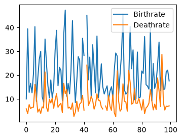
Curves of Birthrate and Deathrate#

df = pd.read_csv("files/countries-of-the-world.csv").sample(100) # sampling 100 lines at random

fig, ax = plt.subplots(figsize=(4,3))
columns = ['Birthrate', 'Deathrate'] 
ax.plot(range(len(df)), df.loc[:,columns[0]], label=columns[0])
ax.plot(range(len(df)), df.loc[:,columns[1]], label=columns[1])
plt.legend()
plt.show()

_images/e2852a011af760ae6369bcc084fa035466ca200d12dbbc6673265317441dbba7.png

Caveat#

Curves are designed to describe the link between two ordered variables
No order in x-axis (counteries)

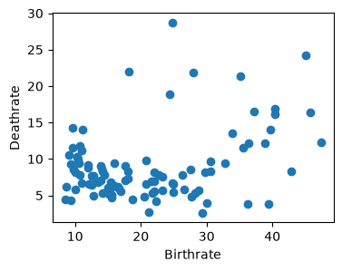
Scatter plot of Birthrate and Deathrate#

fig, ax = plt.subplots(figsize=(4,3))
columns = ['Birthrate', 'Deathrate'] 
ax.scatter(df.loc[:,columns[0]], df.loc[:,columns[1]])
ax.set_xlabel(columns[0]) # name X-axis
ax.set_ylabel(columns[1]) # name y-axis
plt.show()

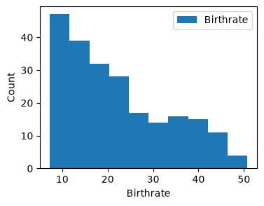
_images/318bda135b00ea73241c12058bb01394001d81519354234100bbc0268aa0c616.png

Plot the histogram of the Birthrate column#

df = pd.read_csv("files/countries-of-the-world.csv")
fig, ax = plt.subplots(figsize=(4,3))
ax.hist(df.loc[:,'Birthrate'], label="Birthrate")
ax.set_xlabel("Birthrate") # Name X-axis
ax.set_ylabel("Count") # Name Y-axis
ax.legend()    
plt.show()

_images/570165146dcfa34f18931a95f63db1e5267e1644674d4e0cd069c146142b565b.png

Plot the histograms of the Birthrate and the Deathrate columns in the same figure#

df = pd.read_csv("files/countries-of-the-world.csv")
fig, ax = plt.subplots(1,1,figsize=(4,3))
ax.hist(df["Birthrate"], alpha=0.5, label='Birthrate') # alpha for transparent colors
ax.hist(df["Deathrate"], alpha=0.5, label='Deathrate') # alpha for transparent colors
ax.set_xlabel('Rate')
ax.set_ylabel('Count')
ax.legend()
plt.show()

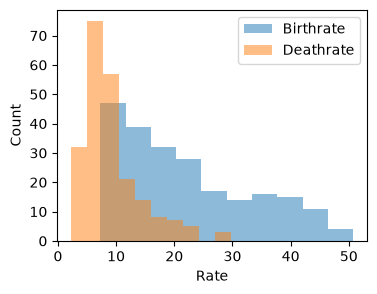
_images/85724e11da7ad78780c0403dd88e02040f071457b528cf4b016b5efdffd2e9c2.png

Note that the bars are not in the same width. This can be solved (but is out of scope)

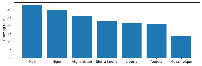
Plots bars of the country’s growing rate (Birthrate - Deathrate) in descending order#

df = pd.read_csv("files/countries-of-the-world.csv").head(7)
fig, ax = plt.subplots(figsize=(10,3))
df=df.loc[:,['Country', 'Birthrate','Deathrate']].dropna(axis=0)
df['Growing rate']=(df.loc[:,'Birthrate']-df.loc[:,'Deathrate'])
df=df.sort_values(by='Growing rate', ascending=False)
ax.bar(df['Country'], df['Growing rate'])
ax.set_ylabel('Growing rate')
plt.show()

_images/16cb290312537e2bb0b1878a567b127259034da79a438d983396cd526c34700d.png

Pandas summary#

We saw how to:#

Create a dataframe (from a file, dict, numpy array)
basic information (head(), tail(), dtypes, info())
Clean the data (add/remove columns/rows, fillna())
Merge tables (concat(), merge())
Analyze the dataset (select rows based on a condition, groupby(), mean(), idxmax(), etc.)
Visualize the data (hist(), plot(), scatter(), boxplot(), bar())

Libraries: Pandas (1.5 weeks)

Contents

Libraries: Pandas (1.5 weeks)#

Python Programming for Engineers#

Tel-Aviv University / 0509-1820 / Fall 2025-2026#

Agenda: Pandas#

Introduction to Pandas#

Basic operations (1)#

Read a dataframe#

[], loc[] and iloc[]#

Do not get confused between df[], df.loc[] and df.iloc[]!#

(3): What will be printed? #

Example: Countries dataset#

Analysis steps#

1. Get basic information (and some more basic operations)#

Read a csv#

Write dataframe to csv#

Print the top 3 rows using the head function#

Note that NaN on the second row!#

2. Data cleaning#

fill missing values#

Option 1: replace nan values with 0 (or any other constant value)#

Option 2: replace nan values with the average of the column#

Option 3: drop all rows that have any NaN value#

Convert Square Miles to Square Kilometers#

Formula: 1 Square Mile =2.58 Square Kilometers#

Add a new column#

A detailed (and longer) version#

Add a new country (row) to the dataframe#

(4): What will be printed? #

NaNs#

(5): What will be printed? #

Delete the Area column#

Delete the country Angola#

Leave only country Angola and Afghanistan#

What will happen if we add ~ before isin ?#

(6): Which countries will be printed?#

Join Tables#

Inner join – consider only the intersection of the tables#

Outer join – consider the union of the table, fill with Nan missing values.#

(7): How many rows in the printed table?#

3. Data analysis#

Which country has the largest population?#

How many countries have more than 1M people?#

How many countries in Oceania have more than 1M peoples?#

Get all countries in the Oceania with Deathrate > 7#

Sort the countries according to the population size#

How to sort countries with the same/NaN population values?#

Break ties according to area size#

groupby#

What is the average population in each region?#

Which country in each region has the largest population?#

Yet, better:#

Print the highest mean Deathrate among all regions#

Self Learning#

Questions from previous exams#

4. Data visualization#

Reminder from the lecture:#

Code template for drawing a figure#

Objective: visualize Birthrate and Deathrate#

Curves of Birthrate and Deathrate#

Caveat#

Scatter plot of Birthrate and Deathrate#

Plot the histogram of the Birthrate column#

Plot the histograms of the Birthrate and the Deathrate columns in the same figure#

Plots bars of the country’s growing rate (Birthrate - Deathrate) in descending order#

Pandas summary#

We saw how to:#

For more info visit the pandas documentation website.#

`[]`, `loc[]` and `iloc[]`#

Do not get confused between `df[]`, `df.loc[]` and `df.iloc[]`!#

Print the top 3 rows using the `head` function#

What will happen if we add `~` before `isin` ?#

`groupby`#